Excerpted from Embedded Control Systems in C/C++
1.1 Introduction
A control system (also called a controller) manages a system’s operation so that the system’s response approximates commanded behavior. A common example of a control system is the cruise control in an automobile: The cruise control manipulates the throttle setting so that the vehicle speed tracks the commanded speed provided by the driver.
In years past, mechanical or electrical hardware components performed most control functions in technological systems. When hardware solutions were insufficient, continuous human participation in the control loop was necessary.
In modern system designs, embedded processors have taken over many control functions. A well-designed embedded controller can provide excellent system performance under widely varying operating conditions. To ensure a consistently high level of performance and robustness, an embedded control system must be carefully designed and thoroughly tested.
This book presents a number of control system design techniques in a step-by-step manner and identifies situations where the application of each is appropriate. It also covers the process of implementing a control system design in C or C++ in a resource-limited embedded system. Some useful approaches for thoroughly testing control system designs are also described.
There is no assumption of prior experience with control system engineering. The use of mathematics will be minimized and explanations of mathematically complex issues will appear in boxed sections. Study of those sections is recommended, but is not required for understanding the remainder of the book. The focus is on presenting control system design and testing procedures in a format that lets you put them to immediate use.
This chapter introduces the fundamental concepts of control systems engineering and describes the steps of designing and testing a controller. It introduces the terminology of control system design and shows how to interpret block diagram representations of systems.
Many of the techniques of control system engineering rely on mathematical manipulations of system models. The easiest way to apply these methods is to use a good control system design software package such as the MATLAB® Control System Toolbox. MATLAB and related products such as Simulink® and the Control System Toolbox are used in later chapters to develop system models and apply control system design techniques.
Throughout this book, words and phrases that appear in the Glossary are displayed in italics the first time they appear.
1.2 Chapter Objectives
After reading this chapter you should be able to:
- Describe the basic principles of feedback control systems.
- Recognize the significant characteristics of a plant (a system to be controlled) as they relate to control system design.
- Describe the two basic steps in control system design: Controller structure selection and parameter specification.
- Develop control system performance specifications.
- Understand the concept of system stability.
- Describe the principal steps involved in testing a control system design.
1.3 Feedback Control Systems
The goal of a controller is to move a system from its initial condition to a desired state and, once there, maintain the desired state. For the cruise control mentioned earlier, the initial condition is the vehicle speed at the time the cruise control is engaged. The desired state is the speed setting supplied by the driver. The difference between the desired and actual state is called the error signal. It is also possible that the desired state will change over time. When this happens, the controller must adjust the state of the system to track changes in the desired state.
A control system that attempts to keep the output signal at a constant level for long periods of time is called a regulator. In a regulator, the desired output value is called the set point. A control system that attempts to track an input signal that changes frequently (perhaps continuously) is called a servomechanism.
Some examples will help clarify the control system elements in familiar systems. Control systems typically have a sensor that measures the output signal to be controlled and an actuator that changes the system’s state in a way that affects the output signal. As Table 1.1 shows, many control systems are implemented using simple sensing hardware that turns an actuator such as a valve or switch on and off.
|
System |
Sensor |
Actuator |
|
Home heating system |
Temperature sensor |
Furnace on/off switch |
|
Automotive engine temperature control |
Thermostat |
Thermostat |
|
Toilet tank water level control |
Float |
Valve operated by float |
Table 1.1 Some Common Control Systems
The systems shown in Table 1.1 are some of the simplest applications of control systems. More advanced control system applications appear in the fields of automotive, aerospace, chemical processing, and in many other areas. This book focuses on the design and implementation of control systems in complex applications.
Comparison of Open Loop Control and Feedback Control
In many control system designs, it is possible to use either open loop control or feedback control. Feedback control systems measure the system parameter being controlled and use that information to determine the control actuator signal. Open loop systems do not use feedback. All the systems described in Table 1.1 use feedback control. The example below demonstrates why feedback control is the nearly universal choice for control system applications.
Consider a home heating system consisting of a furnace and a controller that cycles the furnace off and on to maintain a desired room temperature. Let’s look at how this type of controller could be implemented using open loop control and feedback control.
Open Loop Control: For a given combination of outdoor temperature and desired indoor temperature, it is possible to experimentally determine the ratio of furnace on time to off time that maintains the desired indoor temperature. Suppose a repeated cycle of 5 minutes of furnace on and 10 minutes furnace off produces the desired indoor temperature for a specific outdoor temperature. An open loop controller implementing this algorithm will produce the desired results only so long as the system and environment remain unchanged. If the outdoor temperature changes or if the furnace airflow changes because the air filter was replaced, the desired indoor temperature will no longer be maintained. This is clearly an unsatisfactory design.
Feedback Control: A feedback controller for this system measures the indoor temperature and turns the furnace on when the temperature drops below a turn-on threshold. The controller turns the furnace off when the temperature reaches a higher turn-off threshold. The threshold temperatures are set slightly above and below the desired temperature to keep the furnace from rapidly cycling on and off. This controller adapts automatically to outside temperature changes and to changes in system parameters such as airflow.
This book focuses on control systems that use feedback. This is because feedback controllers, in general, provide superior system performance in comparison to open loop controllers.
While it is possible to develop very simple feedback control systems through trial and error, for more complex applications the only feasible approach is the application of design methods that have been proven over time. This book covers a number of control system design methods and shows you how to employ them directly. The emphasis is on understanding the input and results of each technique, without requiring a deep understanding of the mathematical basis for the method.
As the applications of embedded computing expand, an increasing number of controller functions are moving to software implementations. To function as a feedback controller, an embedded processor uses one or more sensors to measure the system state and drives one or more actuators that change the system state. The sensor measurements are inputs to a control algorithm that computes the actuator commands. The control system design process encompasses the development of a control algorithm and its implementation in software along with related issues such as the selection of sensors, actuators, and the sampling rate.
The design techniques described in this book can be used to develop mechanical and electrical hardware controllers, as well as software controller implementations. This approach allows you to defer the decision of whether to implement a control algorithm in hardware or software until after its initial design has been completed.
1.4 Plant Characteristics
In the context of control systems, a plant is a system to be controlled. From the controller’s point of view, the plant has one or more outputs and one or more inputs. Sensors measure the plant outputs and actuators drive the plant inputs. The behavior of the plant itself can range from trivially simple to extremely complex. At the beginning of a control system design project, it is helpful to identify a number of plant characteristics relevant to the design process.
Linear and Nonlinear Systems
A linear plant model is required for some of the control system design techniques covered in following chapters. In simple terms, a linear system produces an output that is proportional to its input. Small changes in the input signal result in small changes in the output. Large changes in the input cause large changes in output. A truly linear system must respond proportionally to any input signal, no matter how large. Note that this proportionality could also be negative: A positive input might produce a proportional negative output.
Definition of a Linear System
Consider a plant with one input and one output. Suppose you run the system for a period of time while recording the input and output signals. Call the input signal u1(t) and the output signal y1(t). Perform this experiment again with a different input signal. Name the input and output signals from this run u2(t) and y2(t) respectively. Now perform a third run of the experiment with the input signal u3(t) = u1(t) + u2(t).
The plant is linear if the output signal y3(t) = y1(t) + y2(t) for any arbitrarily selected input signals u1(t) and u2(t).
Real world systems are never precisely linear. Various factors always exist that introduce nonlinearities into the response of a system. For example, some nonlinearities in the automotive cruise control discussed earlier are:
- The force of air drag on the vehicle is proportional to the square of its speed through the air.
- Friction (a nonlinear effect) exists within the drive train and between the tires and road.
- The speed of the vehicle is limited to a range between minimum and maximum values.
However, the linear idealization is extremely useful as a tool for system analysis and control system design. Several of the design methods in the following chapters require a linear plant model. This immediately raises a question: If you do not have a linear model of your plant, how do you obtain one?
The approach usually taught in engineering courses is to develop a set of mathematical equations based on the laws of physics as they apply to the operation of the plant. These equations are often nonlinear, in which case it is necessary perform additional steps to linearize them. This procedure requires intimate knowledge of plant behavior as well as a strong mathematical background.
In this book, we don’t assume this type of background. Our focus is on simpler methods of acquiring a linear plant model. For instance, if you need a linear plant model but don’t want to develop one, you can always let someone else do it for you. Linear plant models are sometimes available from system data sheets or by request from experts familiar with the mathematics of a particular type of plant. Another approach is to perform a literature search to locate linear models of plants similar to the one of interest.
System identification is an alternative if none of the above approaches are suitable. System identification is a technique for performing semi-automated linear plant model development. This approach uses recorded plant input signals and output signals data to develop a linear system model that best fits the input and output data. System identification is discussed further in Chapter 3.
Simulation is another technique for developing a linear plant model. You can develop a nonlinear simulation of your plant using a tool such as Simulink and derive a linear plant model based on the simulation. We will apply this approach in some of the examples presented in later chapters.
Perhaps you just don’t want to expend the effort required to develop a linear plant model. With no plant model, an iterative procedure must be used to determine a suitable controller structure and parameter values. Chapter 2 discusses procedures for applying and tuning PID controllers. PID controller tuning is carried out using the results of experiments performed on the system consisting of plant plus controller.
Time Delays
Sometimes a linear model accurately represents the behavior of a plant, but a time delay exists between an actuator input and the start of the plant response to the input. This does not refer to sluggishness in the plant’s response. A time delay exists only when there is absolutely no response for some time interval following a change to the plant input.
For example, a time delay occurs when controlling the temperature of a shower. Changes in the hot or cold water valve positions do not have immediate results. There is a delay while water with the adjusted temperature flows up to the shower head and then down onto the shower-taker. Only then does feedback exist to indicate if further temperature adjustments are needed.
Many industrial processes exhibit time delays. Control system design methods that rely on linear plant models can’t directly work with time delays, but it is possible to extend a linear plant model to simulate the effects of a time delay. The resulting model is also linear and captures the approximate effects of the time delay. Linear control system design methods are applicable to the extended plant model. Time delays will be discussed further in Chapter 3.
Continuous-Time and Discrete-Time Systems
A continuous-time system has outputs with values defined at all points in time. The outputs of a discrete-time system are only updated or used at discrete points in time. Real world plants are usually best represented as continuous-time systems. In other words, these systems have measurable parameters such as speed, temperature, weight, etc. defined at all points in time.
The discrete-time systems of interest in this book are embedded processors and their associated input/output (I/O) devices. An embedded computing system measures its inputs and produces its outputs at discrete points in time. The embedded software typically runs at a fixed sampling rate, which results in input and output device updates at equally spaced points in time.
I/O Between Discrete-Time Systems and Continuous-Time Systems
A class of I/O devices interfaces discrete-time embedded controllers with continuous plants by performing direct conversions between analog voltages and the digital data values used in the processor. The analog to digital converter (ADC) performs input from an analog plant sensor to a discrete-time embedded computer. Upon receiving a conversion command, the ADC samples its analog input voltage and converts it to a quantized digital value. The behavior of the analog input signal between samples is unknown to the embedded processor.
The digital to analog converter (DAC) converts a quantized digital value to an analog voltage, which drives an analog plant actuator. The output of the DAC remains constant until it is updated at the next control algorithm iteration.
Two basic approaches are available for developing control algorithms that run as discrete-time systems. The first is to perform the design entirely in the discrete-time domain. For design methods that require a linear plant model, this method requires conversion of the continuous-time plant model to a discrete-time equivalent. One drawback of this approach is that it is necessary to specify the sampling rate of the discrete-time controller at the very beginning of the design process. If the sampling rate changes, all the steps in the control algorithm development process must be repeated to compensate for the change.
An alternative procedure is to perform the control system design in the continuous-time domain followed by a final step to convert the control algorithm to a discrete-time representation. Using this method, changes to the sampling rate only require repetition of the final step. Another benefit of this approach is that the continuous-time control algorithm can be implemented directly in analog hardware, if that turns out to be the best solution for a particular design. A final benefit of this approach is that the methods of control system design tend to be more intuitive in the continuous-time domain than in the discrete-time domain.
For these reasons, the design techniques covered in this book will be based in the continuous-time domain. Chapter 8 will discuss the conversion of a continuous-time control algorithm to an implementation in a discrete-time embedded processor using the C/C++ programming languages.
Number of Inputs and Outputs
The simplest feedback control system has one input and one output, and is called a single-input-single-output (SISO) system. In a SISO system, a sensor measures one signal and the controller produces one signal to drive an actuator. All of the design procedures in this book are applicable to SISO systems.
Control systems with more than one input or output are called MIMO systems, meaning multiple-input-multiple-output systems. Because of the added complexity, fewer MIMO system design procedures are available. Only the pole placement and optimal control design techniques (covered in Chapters 5 and 6) are directly suitable for MIMO systems. Chapter 7 covers issues specific to MIMO control system design.
In many cases, MIMO systems can be decomposed into a number of approximately equivalent SISO systems. For example, flying an aircraft requires simultaneous operation of several independent control surfaces including the rudder, ailerons, and elevator. This is clearly a MIMO system, but focusing on a particular aspect of behavior can result in a SISO system for control system design purposes. For instance, assume the aircraft is flying straight and level and must maintain a desired altitude. A SISO system for altitude control uses the measured altitude as its input and the commanded elevator position as its output. In this situation, the sensed parameter and the controlled parameter are directly related and have little or no interaction with other aspects of system control.
The critical factor that determines whether a MIMO system is suitable for decomposition into a number of SISO systems is the degree of coupling between inputs and outputs. If changes to a particular plant input result in significant changes to only one of its outputs, it is probably reasonable to represent the behavior of that input-output signal pair as a SISO system. When use of this technique is appropriate, all of the SISO control system design approaches become available for use with the system.
However, when too much coupling exists from a plant input to multiple outputs, there is no alternative but to perform a control system design using a MIMO method. Even in systems with weak cross coupling, the use of a MIMO design procedure will generally produce a superior design compared to the multiple SISO designs developed assuming no cross coupling between input-output signal pairs.
1.5 Controller Structure and Design Parameters
The two fundamental steps in designing a controller are:
- Specify the controller structure.
- Determine the value of the design parameters within that structure.
The controller structure identifies the inputs, outputs, and mathematical form of the control algorithm. Each controller structure contains one or more adjustable design parameters. Given a controller structure, the control system designer must select a value for each parameter so that the overall system (consisting of the plant and the controller) satisfies performance requirements.
For example, in the root locus method described in Chapter 4, the controller structure might produce an actuator signal computed as a constant (called the gain) times the error signal. The adjustable parameter in this case is the value of the gain.
Like engineering design in other domains, control system design tends to be an iterative process. During the initial controller design iteration, it is best to begin with the simplest controller structure that could possibly provide adequate performance. Then, using one or more of the design methods in the following chapters, the designer attempts to identify values for the controller parameters that result in acceptable system performance.
It may turn out that no combination of parameter values for a given controller structure results in satisfactory performance. When this happens, the controller structure must be altered in some way to enable performance goals to be met. The designer then determines values for the adjustable parameters of the new structure. The cycle of controller structure modification and design parameter selection repeats until a final design with acceptable system performance has been achieved.
The following chapters contain several examples demonstrating the application of this two-step procedure using different control system design techniques. The examples come from engineering domains where control systems are regularly applied. Studying the steps in each example will help you develop an understanding of how to select an appropriate controller structure. For some of the design techniques, the determination of design parameter values is an automated process using control system design software. For the other design methods, you must follow the appropriate steps to select values for the design parameters.
Following each iteration of the two-step design procedure, you must evaluate the resulting controller to see if it meets performance requirements. Chapter 9 covers techniques for testing control system designs, including simulation testing and tests of the controller operating in conjunction with the actual plant.
1.6 Block Diagrams
A block diagram of a plant and controller is a graphical means to represent the structure of a controller design and its interaction with the plant. Figure 1.1 is a block diagram of an elementary feedback control system. Each block in the figure represents a system component. The solid lines with arrows indicate the flow of signals between the components.
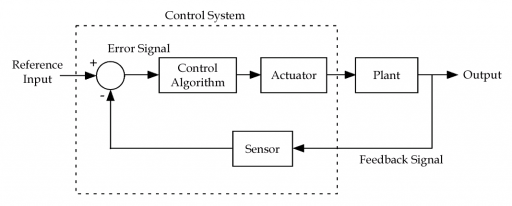
Figure 1.1 Block diagram of a feedback control system
In block diagrams of SISO systems, a solid line represents a single scalar signal. In MIMO systems, a single line may represent multiple signals. The circle in the figure represents a summing junction, which combines its inputs by addition or subtraction depending on the + and – signs next to each input.
The contents of the dashed box in Fig. 1.1 are the control system components. The controller inputs are the reference input (also called a set point) and the plant output signal (measured by the sensor), which is used as feedback. The controller output is the actuator signal that drives the plant.
A block in a diagram can represent something as simple as a constant value that multiplies the block input, or as complex as a nonlinear system with no known mathematical representation. The design techniques in Chapter 2 do not require a model of the Plant block in Fig. 1.1, but the methods in the subsequent chapters will require a linear model of the plant.
Linear System Block Diagram Algebra
It is possible to manipulate block diagrams containing only linear components to achieve compact mathematical expressions representing system behavior. The goal of this manipulation is to determine the system output as a function of its input. The expression resulting from this exercise is useful in various control system analysis and design procedures.
Each block in the diagram must represent a linear system expressed in the form of a transfer function. Transfer functions are introduced in Chapter 3. Knowledge of the details of transfer functions is not required to perform block diagram algebra.
Figure 1.2 is a block diagram of a simple linear feedback control system. Lower case characters identify the signals in this system.
- r is the reference input, also called the set point.
- e is the error signal, computed by subtracting the sensor measurement from the reference input.
- y is the system output, which is measured and used as the feedback signal.
The blocks in the diagram represent linear system components. Each block can represent dynamic behavior with any degree of complexity as long as the requirement of linearity is satisfied.
- Gc is the linear controller algorithm.
- Gp is the linear plant model (including actuator dynamics.)
- H is a linear model of the sensor, which can be modeled as a constant such as 1 if the sensor dynamics are negligible.
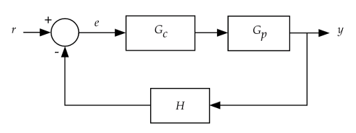
Figure 1.2 Linear feedback control system.
The fundamental rule of block diagram algebra states that the output of a block equals the block input multiplied by the block transfer function. Applying this rule twice results in Eq. 1.1. In words, Eq. 1.1 says the system output y is the error signal e multiplied by the controller transfer function Gc, and then multiplied again by the plant transfer function Gp.
(1.1)
![]()
Block diagram algebra obeys the usual rules of algebra. Multiplication and addition are commutative, so the parentheses in Eq. 1.1 are unnecessary. This also means that the positions of the Gc and Gp blocks in Fig. 1.2 can be swapped without altering the external behavior of the system.
The error signal e is the output of a summing junction subtracting the sensor measurement from the reference input r. The sensor measurement is the system output y multiplied by the sensor transfer function H. This relationship appears in Eq. 1.2.
(1.2)
![]()
Substituting Eq. 1.2 into Eq. 1.1 and rearranging algebraically results in Eq. 1.3.
(1.3)
![]()
Equation 1.3 is a transfer function giving the ratio of the system output to its reference input. This form of system model is suitable for use in numerous control system analysis and design tasks.
Using the relation of Eq. 1.3, the entire system in Fig. 1.2 can be replaced by the equivalent system shown in Fig. 1.3. Remember, these manipulations are only valid when the components of the block diagram are all linear.
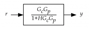
Figure 1.3 Equivalent system to the system shown in Fig. 1.2.
1.7 Performance Specifications
One of the first steps in the control system development process is the definition of a suitable set of system performance specifications. Performance specifications guide the design process and provide the means for determining when a controller design is satisfactory. Controller performance specifications can be stated in both the time domain and in the frequency domain.
Time domain specifications usually relate to performance in response to a step change in the reference input. An example of such a step input is instantaneously changing the reference input from 0 to 1. Time domain specifications include, but are not limited to, the following parameters [1]:
- Rise time from 10% to 90% of the commanded value, tr.
- Time to peak magnitude, tp.
- Peak magnitude, Mp. This is often expressed as the peak percentage by which the output signal overshoots the step input command.
- Settling time to within some fraction (such as 1%) of the step input command value, ts.
Examples of these parameters appear in Fig. 1.4. This figure shows the response of a hypothetical plant plus controller to a step input command with an amplitude of one. The time axis zero location is the instant of application of the step input.
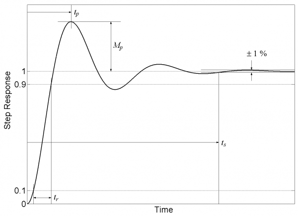
Figure 1.4 Time domain control system performance parameters.
The step response in Fig. 1.4 represents a system with a fair amount of overshoot (in terms of Mp) and oscillation before converging to the reference input. Sometimes the step response has no overshoot at all. When no overshoot occurs, the tp parameter becomes meaningless and Mp is zero.
Tracking error is the error in the output that remains after the input function has been applied for a long time and all transients have died out. It is common to specify the steady-state controller tracking error characteristics in response to different commanded input functions such as steps, ramps, and parabolas.
Here are some example specifications of tracking error in response to different input functions:
- Zero tracking error in response to a step input.
- Less than X tracking error magnitude in response to a ramp input, where X is some nonzero value.
In addition to the time domain specifications discussed above, performance specifications can be specified in the frequency domain. The controller reference input is usually a low frequency signal, while noise in the sensor measurement used by the controller often contains high frequency components. It is normally desirable for the control system to suppress the high frequency components related to sensor noise while responding to changes in the reference input. Performance specifications capturing these low and high frequency requirements would look similar to these:
- For sinusoidal reference input signals with frequencies below a cutoff point, the amplitude of the closed loop (plant plus controller) response must be within X% of the commanded amplitude.
- For sinusoidal reference input signals with frequencies above a higher cutoff point, the amplitude of the closed loop response must be reduced by at least Y%.
In other words, the frequency domain performance requirements given above say that the system response to expected changes in the reference input must be acceptable while simultaneously attenuating the effects of noise in the sensor measurement. Looked at in this way, the closed loop system exhibits the characteristics of a lowpass filter.
Frequency domain performance specifications will be discussed in more detail in Chapter 4.
1.8 System Stability
Stability is a critical issue throughout the control system design process. A stable controller produces appropriate responses to changes in the reference input. If the system stops responding properly to changes in the reference input and does something else instead, it has become unstable.
Figure 1.5 shows an example of unstable system behavior. The initial response to the step input overshoots the commanded value by a large amount. The response to that overshoot is an even larger overshoot in the other direction. This pattern continues, with increasing output amplitude over time. In a real system, an unstable oscillation like this grows in amplitude until some nonlinearity such as actuator saturation (or a system breakdown!) limits the response.
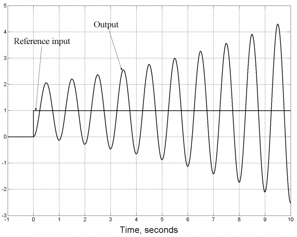
Figure 1.5 System with an unstable oscillatory response.
System instability is a risk when using feedback control. Avoiding instability is an important part of the control system design process.
In addition to achieving a bare minimum degree of stability, a control system must possess a degree of robustness. A robust controller can tolerate limited changes to the parameters of the plant and its operating environment while continuing to provide satisfactory, stable performance. For example, an automotive cruise control must maintain the desired vehicle speed by adjusting the throttle position in response to changes in road grade (an environmental change.) The cruise control must also perform properly whether or not the vehicle is pulling a trailer (a change in system parameters.)
Determining the allowable ranges of system and environmental parameter changes is part of the controller specification and design process. To demonstrate robustness, the designer must evaluate controller stability under worst-case combinations of expected plant and environment parameter variations. For each combination of parameter values, a robust controller must satisfy all of its performance requirements.
When working with linear models of plants and controllers it is possible to precisely determine whether a particular plant and controller form a stable system. Chapter 3 describes how to determine linear system stability.
If no mathematical model for the plant exists, stability can only be evaluated by testing the plant and controller under a variety of operating conditions. Chapter 2 covers techniques for developing stable control systems without the use of a plant model. Chapter 9 describes methods for performing thorough control system testing.
1.9 Control System Testing
Testing is an integral part of the control system design process. Many of the design methods in this book rely on the use of a linear plant model. Creating a linear model always involves approximation and simplification of the true plant behavior. The implementation of a controller using an embedded processor introduces nonlinear effects such as quantization. As a result, both the plant and the controller contain nonlinear effects that are not accounted for in a linear control system design.
The ideal way to demonstrate correct operation of the nonlinear plant and controller over the full range of system behavior is by performing thorough testing with an actual plant. This type of system-level testing normally occurs late in the product development process when prototype hardware becomes available. Problems found at this stage of the development cycle tend to be very expensive to fix.
Because of this, it is highly desirable to perform thorough testing at a much earlier stage of the development cycle. Early testing enables discovery and repair of problems when they are relatively easy and inexpensive to fix. However, testing the controller early in the product development process may not be easy if a prototype plant does not exist on which to perform tests.
System simulation provides a solution to this problem [2]. A simulation containing detailed models of the plant and controller is extremely valuable for performing early-stage control system testing. This simulation should include all relevant nonlinear effects present in the actual plant and controller implementations. While the simulation model of the plant must necessarily be a simplified approximation of the actual system, it should be a much more authentic representation than the linear plant model used in the controller design.
When using a simulation in a product development process, it is imperative to perform thorough simulation verification and validation.
- Verification demonstrates the simulation has been implemented correctly according to its design specifications.
- Validation demonstrates that the simulation accurately represents the behavior of the simulated system and its environment for the intended purposes of the simulation.
The verification step is relevant for any software development process, and simply shows that the software performs as its designers intended. In simulation work, verification can occur in the early stages of a product development project. It is possible (and common) to perform verification for a simulation of a system that does not yet exist. This consists of making sure that the models used in the simulation are correctly implemented and produce the expected results. Verification allows the construction and application of a simulation in the earliest phases of a product development project.
Validation is a demonstration that the simulation models the embedded system and the real world operational environment with acceptable accuracy. A standard approach for validation is to use the results of system operational tests for comparison against simulation results. This involves running the simulation in a scenario that is identical to a test that was performed by the actual system in a real world environment. The results of the two tests are compared and the differences are analyzed to determine if they represent significant deviations between the simulation and the actual system.
A drawback of this approach to validation is that it cannot happen until a complete system prototype is available. Even when a prototype does not exist, it may be possible to perform validation at an earlier project phase at the component and subsystem level. You can perform tests on those system elements in a laboratory environment and duplicate the tests with the simulation. Comparing the results of the two tests provides confidence in the validity of the component or subsystem model.
The use of system simulation is common in the control engineering world. If you are unfamiliar with the tools and techniques of simulation, see reference [2] for an introduction to this topic.
1.10 Computer-Aided Control System Design
The classical control system analysis and design methods discussed in Chapter 4 were originally developed and have been taught for years as techniques that rely on hand-drawn sketches. While this approach leads to a level of design intuition in the student, it takes significant time and practice to develop the necessary skills.
Since this book intends to enable the reader to rapidly apply a variety of control system design techniques, automated approaches will be emphasized rather than manual methods. Several software packages are commercially available that perform control system analysis and design functions as well as complete nonlinear system simulation. Some examples are listed below.
- VisSim/Analyze. This product performs linearization of nonlinear plant models and supports compensator design and testing. This is an add-on to the VisSim product, which is a tool for performing modeling and simulation of complex dynamic systems. For more information see https://vissim.com/products/addons/analyze.html.
- Mathematica Control System Professional. This tool handles linear SISO and MIMO system analysis and design in the time and frequency domains. This is an add-on to the Mathematica product. Mathematica provides an environment for performing symbolic and numerical mathematical computations and programming. For more information see https://wolfram.com/products/applications/control/.
- MATLAB Control System Toolbox. This is a collection of algorithms that implement common control system analysis, design and modeling techniques. It covers classical design techniques as well as modern state-space methods. This is an add-on to the MATLAB product, which integrates mathematical computing, visualization, and a programming language to enable the development and application of sophisticated algorithms to large sets of data. For more information see https://mathworks.com/products/control/.
This book uses MATLAB, the Control System Toolbox, and other MATLAB add-on products to demonstrate a variety of control system modeling, design, and simulation techniques. These tools provide efficient, numerically robust algorithms to solve a variety of control system engineering problems. The MATLAB environment also provides powerful graphics capabilities for displaying the results of control system analysis and simulation procedures.
The MATLAB software is not cheap, but powerful tools like this seldom are. Pricing information is available online at https://mathworks.com/store/index.html. MATLAB products are available for a free 30-day trial period. If you are a student using the software in conjunction with courses at a degree-granting institution, you are entitled to purchase the MATLAB Student Version and Control System Toolbox at a greatly reduced price. For more information, see https://mathworks.com/products/studentversion/buy_now.shtml.
1.11 Summary
Feedback control systems measure attributes of the system being controlled and use that information to determine the control actuator signal. Feedback control provides superior performance compared to open loop control when environmental or system parameters change.
The system to be controlled is called a plant. Some of the characteristics of the plant as it relates to the control system design process are:
- Linearity. A linear plant representation is required for some of the design methods presented in following chapters. All real world systems are nonlinear, but it is often possible to develop a suitable linear approximation of a plant.
- Continuous-time or discrete-time. A continuous-time system is usually the best way to represent a plant. Embedded computing systems function in a discrete-time manner. Input-output devices such as DACs and ADCs are the interfaces between a continuous-time plant and a discrete-time controller.
- Number of input and output signals. A plant that has a single input and a single output is a SISO system. If it has more than one input or output it is a MIMO system. MIMO systems can often be approximated as a set of SISO systems for design purposes.
- Presence of time delays. Time delays in a plant add some difficulty to the problem of designing a controller.
The two fundamental steps in control system design are:
- Specify the controller structure.
- Determine the value of the design parameters within that structure.
The control system design process usually involves the iterative application of these two steps. In the first step, a candidate controller structure is selected. In the second step, a design method is used to determine suitable parameter values for that structure. If the resulting system performance is inadequate, the cycle is repeated with a new, usually more complex, controller structure.
A block diagram of a plant and controller graphically represents the structure of a controller design and its interaction with the plant. It is possible to perform algebraic operations on the components of a block diagram to reduce the diagram to a simpler form.
Performance specifications guide the design process and provide the means for determining when controller performance is satisfactory. Controller performance specifications can be stated in both the time domain and the frequency domain.
Stability is a critical issue throughout the control system design process. A stable controller produces appropriate system responses to changes in the reference input. Stability evaluation must be performed as part of the analysis of a controller design.
Testing is an integral part of the control system design process. It is highly desirable to perform thorough control system testing at an early stage of the development cycle, but prototype system hardware may be unavailable at that time. As an alternative, a simulation containing detailed models of the plant and controller is useful for performing early-stage control system testing. When prototype hardware is available, thorough testing of the control system across the intended range of operating conditions is imperative.
Several software packages are commercially available that perform control system analysis and design functions as well as complete nonlinear system simulation. These tools can significantly speed the steps of the control system design and analysis processes. This book will emphasize the application of the MATLAB Control System Toolbox and other MATLAB-related products to control system design, analysis, and system simulation tasks.
Excerpted from Embedded Control Systems in C/C++